As pointed out in class, Helmholtz coils are two current loops in parallel with spacing equal to their radii. You might also want to look at the material presented below.
See the Helmholtz coils built by former honors students for the IU group in the GlueX Experiment
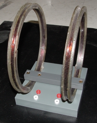
Here are the coils you will use:
A copy of the Gaussmeter manual [gm1a_gaussmeter.pdf] will be in the lab. Please do not print out multiple copies but you may want to view the PDF copy online. More information on the gaussmeter here.

- Based on the dimensions of the coil and the number of turns and the current estimate the field at the center of a single energized coil.
- Measure the field and compare with your expectations
- Due to the same for the other coil (the coils should be identical)
- For a single energized coil measure the field along the axis on either side of the coil. Compare B(z) with theoretical expectations.
- Compare the field for some point on the axis at a distance from the center corresponding to several radii to the field a same distance from the coil center but in the plane of the coil.
- Now estimate the field at the midpoint between two coils with both coils energized.
- Measure the field on axis out to a distance correponding to at least one radius outside of the coils on either side. Compare your measurements with theoretical expectations.
- Measure the field at the midpoint with currents running in opposite directions.
- Use IGOR to compare data with theory.
Notes
on deriving the Helmholz fields
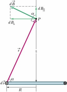
The field on axis for a single loop of current is given by:
Now caculate the field between the two parallel loops, each carrying current I and with N turns per loop.
This arrangement produces a
very uniform field along the axis between the coils. In your text
book Helmholtz coils are described in Problems 50, 53 and 55 of
Chapter 30 and for completeness the solutions are given here:
P30_050.PDF
P30_053.PDF
P30_055.PDF
I suggest you look at these. The field is specified on axis with z measured from the center of one of the loops and the separation between the loops is s.
Now look at the field at the center of the two loops. The first derivative of the above is zero at the center - as are all the odd derivatives. The second derivative is zero at the center if the coil separation is equal to the radius of the loops.
That means that the field is
very uniform - at reasonable distance from the center of the
coils, the field does not change appreciably from its value at the
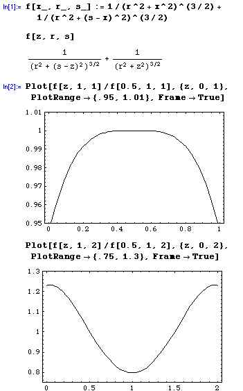
center. I show below a Mathematica calculation of the relative
value of the field between the coils compared to the central
value. I look only at the bracketed part of the above expression.
First I choose:
r = s = 1 and then r = 1 and s = 2. Note that in the first plot
the vertical scale goes from 0.95 to 1.01 and in the second plot
the vertical axis goes from 0.75 to 1.3. So doubling the
separation from the ideal case causes quite a variation in the
field along the zxis.
This Mathematica Notebook [helmholtz.nb] shows you how to calculate the higher order derivatives using the D[f[x],{x,n}] function. The algebra can get messy. And the relevance of the first three derivatives vanishing at the center can be appreciated by considering the Taylor series expansion of the field about the center point. For those who need and intro or a refresher, please look at this website about the Taylor series Derivation.