Sometimes you can cast the solution to a problem in the form
One way to get a numerical answer is to plot y =x and y = F(x) on the same set of axes and find the value of x where the straight line (y=x) and curve (F(x)) intercept - that is the solution.
Another Technique
It can also be solved by the so-called iterative technique. That is, you start with some guess at x, call it x0 and then you get x1:

Using Your Calculator
This is obviously a nice technique to use with your calculator. Key in the expression for F(x) and make some guess at the value of x. Now use this value of x to get a numerical value of F(x). Use this value as your new x and then re-calculate F(x). Keep doing this. Eventually the values you get for F(x) approach the anwer.
Check Out
These nice animations.
Why It Works
The above procedure will converge on the solution - provided that you are operating in a range of x such that:
If the derivative evualated at the solution (x = r) is close to 1 the convergence is slow. If we write the difference between the nth approximation and the solution as:
we can show that:
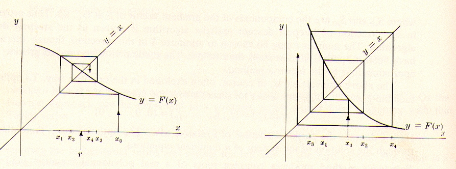
F'(r) is the derivative of F(x) evaluated at x = r. In other words, the difference from the solution decreases. The figures below show the procedure pictorially. For the case on the left the procedure converges but not for the case on the right.
Back in 1225, the great mathematician Leonardo of Pisa (a.k.a. Fibonacci) found the root of:
to be x = 1.368808107. No one seems to know how (or why !) he did this. Use the iterative method to solve this. How many iterations do you need ?

Fibonacci